Tutorial 5 - An advanced cavity example ‘Bessel-Gauss’ cavity

Small introduction

In this tutorial we will design and calculate the eigenmodes of an advanced type of laser cavities called Bessel-Gauss cavities. This class of cavities support Bessel-Gauss beams which offer some interesting properties, for example an extended depth of field with high intensity sometimes called non-diffracting region and annular intensity distribution in the far field. These properties make this class of beams very interesting for several applications such as biomedical imaging, particle trapping, strong-field applications...etc. Well, I hope that this small introduction motivates you to learn more about these cavities. In the tutorial we will take the design studied in this open access paper [Schimpf2012] which is a good one (I find) to learn more about Bessel-Gauss beams and cavities and can be downloaded here ), this way we can compare the results obtained using OpenCavity with those of the paper. Lets start with the scheme of the cavity:

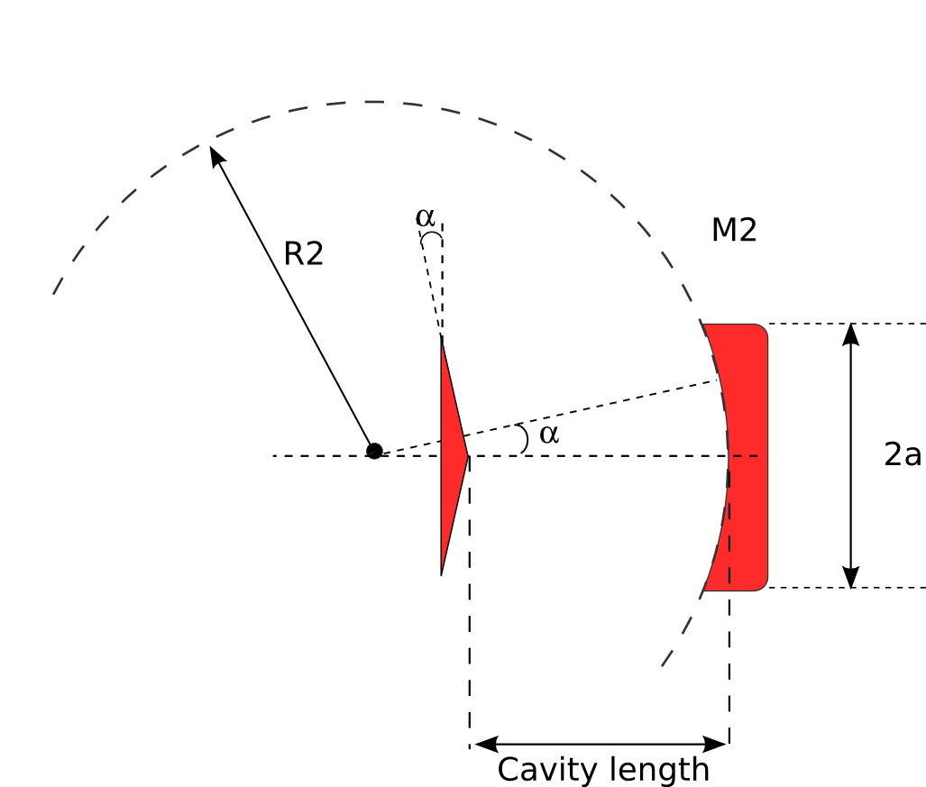
As we can see this cavity contains concave mirror with radius of curvature R2=250mm and a conical reflector with base angle \(\alpha=0.5°\). the cavity length Lc=78mm. This results in a ring-shaped mode with radius of 1.5mm at the first mirror. For more details about how to calculate the stability of such a cavity take a look at the paper. To define this cavity we use general definition using ABCD transfer matrix and a phase mask to introduce the conical phase function, using subsystems cascading as shown in Tutorial 3 - using apertures and phase masks as follows:

Cavity design using OpenCavity

Entering the cavity parameters and transfer matrices of the subsystems

In [1]: import opencavity.modesolver as ms

In [2]: from opencavity.propagators import FresnelProp

In [3]: import numpy as np #import numerical Python

In [4]: import matplotlib.pylab as plt # import matplotlib to plot figures

In [5]: R1=1e18; R2=250*1e3; Lc=78*1e3; npts=1000; a=2700; # cavity parameters

In [6]: M1=np.array([[1,0 ],[-2/R1, 1]]);   #plane mirror M1

In [7]: M2=np.array([[1, Lc],[0, 1]]);  #propagation distance Lc

In [8]: M3=np.array([[1, 0],[-2/R2, 1]]); #concave mirror M2

In [9]: M4=np.array([[1, Lc],[0, 1]]); #propagation distance Lc

In [10]: M11=M2.dot(M1); M22=M4.dot(M3); # sub-system 1 & sub-system 2

In [11]: A11=M11[0,0]; B11=M11[0,1]; C11=M11[1,0]; D11=M11[1,1] # getting the members of subsystem 1 matrix

In [12]: A22=M22[0,0]; B22=M22[0,1]; C22=M22[1,0]; D22=M22[1,1] # getting the members of subsystem 2 matrix

Creating the cavity-subsystems

In [13]: sys1=ms.CavEigenSys(wavelength=1.04); # working wavelength 1.04 micron

In [14]: sys2=ms.CavEigenSys(wavelength=1.04);

In [15]: sys1.build_1D_cav_ABCD(a,npts,A11,B11,C11,D11) #

In [16]: sys2.build_1D_cav_ABCD(a,npts,A22,B22,C22,D22) # to reinitialize the sub-system

Creating the axicon function with base angle =-0.5°, sys.k is the wave vector, and remember that all the fields are not spaced linearly see (Notes on vectors spacing in OpenCavity)

In [17]: theta=-0.5*3.14/180;# reflector is equivalent to refractive axicon with 2 x theta

In [18]: T_axicon=ms.np.exp((1j*sys1.k)*2*theta*(ms.np.sign(sys1.x1))*sys1.x1)

Applying the axicon function and solve and show the modes

In [19]: sys1.apply_mask1D(T_axicon)
Applying 1D Mask...
Mask applied.

In [20]: sys1.cascade_subsystem(sys2)
systems cascaded.

In [21]: sys1.solve_modes()
running the eigenvalues solver...

In [22]: sys1.show_mode(0,what='intensity')

In [23]: sys1.show_mode(0,what='phase')

In [24]: l,tem00=sys1.get_mode1D(0)

In [25]: print 1-np.abs(l)**2 #round trip losses
0.0754566450443

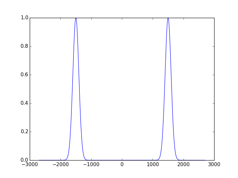
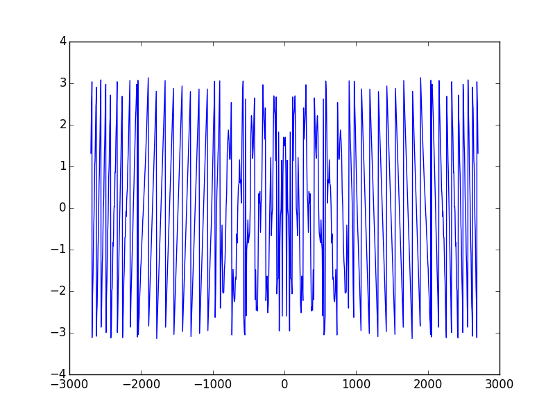
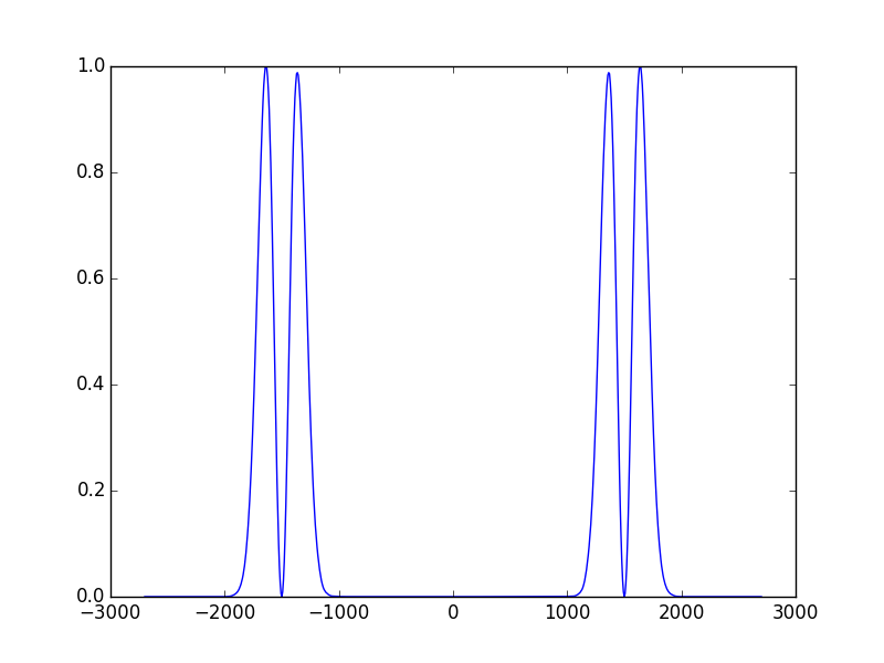
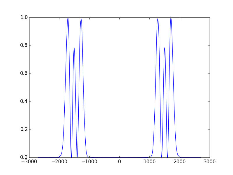
The first thing we can notice is that the mode contains two lobes, this is because it has a ring-shaped intensity distribution. And the second thing is the conical component in the phase. The obtained mode is identical to the result of paper (Fig 6-a) and the lobe spacing is the one we expected :1.5mm (1500 micron in the figure). Lets see the high order modes to complete the results of the (Fig 6).

In [26]: sys1.show_mode(2,what='intensity')

In [27]: sys1.show_mode(4,what='intensity')

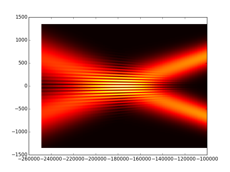
To see the high intensity region of these beams we use the FresnelProp() module presented in Tutorial 4 - Calculating the output beam, but this time we use a new function propsys.yz_prop_chart(z_min,z_max,n_step,x) that calculates the propagated beam in n_step successive planes from z_min to z_max and x is the planes abscissa. However in this cavity arrangement the mode has already ring-shape at the first plane and is diverging, thus the high intensity region is behind the beam so to see it we enter negative propagation distance (to follow the paper), obviously this does not have physical meaning in real word but mathematically it means that we merely invert the time axis, or to consider a beam propagating from the right to the left.

In [28]: propsys=FresnelProp() # create a propagator object

In [29]: propsys.set_start_beam(tem00, sys1.x1)

In [30]: d=-172.0e3

In [31]: M=ms.np.array([[1,d ],[0, 1]]);

In [32]: propsys.set_ABCD(M)

In [33]: propsys.yz_prop_chart(-250e3,-100e3,100,sys1.x1/2) # z_min=-250, z_max=-100, n_planes=100

In [34]: plt.set_cmap('hot')

In [35]: propsys.show_prop_yz()

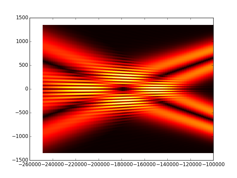
# propagate the second mode
In [36]: l,tem02=sys1.get_mode1D(2)

In [37]: propsys.set_start_beam(tem02, sys1.x1)

In [38]: propsys.yz_prop_chart(-250e3,-100e3,100,sys1.x1/2)

In [39]: propsys.show_prop_yz()

# propagate the third mode
In [40]: l,tem03=sys1.get_mode1D(4)

In [41]: propsys.set_start_beam(tem03, sys1.x1)

In [42]: propsys.yz_prop_chart(-250e3,-100e3,100,sys1.x1/2)

In [43]: propsys.show_prop_yz()

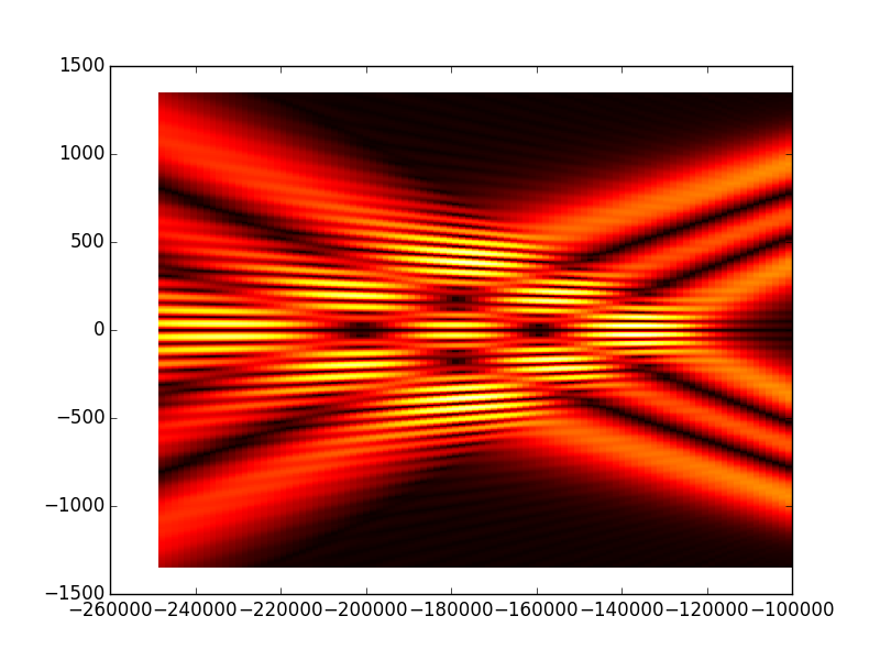
NB: As we are using Fresnel propagation method we can not calculate the propagation over small distances because this will break the paraxial condition (small angles from the propagation axis) see (to add in the first part ‘before starting’). What we observe is that the high intensity region is behind the conical mirror, after that the beam takes an annular shape and diverges as it propagates. In the next tutorial we will change the cavity design to have the high intensity region after the concave mirror.

The cleaned code

# -*- coding: utf-8 -*-

import opencavity.modesolver as ms
from opencavity.propagators import FresnelProp
import numpy as np #import numerical Python 

R1=1e18; R2=250*1e3; Lc=78*1e3; npts=1000; a=2700; # cavity parameters
M1=np.array([[1,0 ],[-2/R1, 1]]);   #concave mirror M1 
M2=np.array([[1, Lc],[0, 1]]);  #propagation distance Lc
M3=np.array([[1, 0],[-2/R2, 1]]); #concave mirror M2
M4=np.array([[1, Lc],[0, 1]]); #propagation distance Lc
M=M4.dot(M3).dot(M2).dot(M1) # calculating the global matrix (note the inversed order)

M11=M2.dot(M1); M22=M4.dot(M3); # sub-system 2 
A11=M11[0,0]; B11=M11[0,1]; C11=M11[1,0]; D11=M11[1,1] # getting the members of subsystem 1 matrix
A22=M22[0,0]; B22=M22[0,1]; C22=M22[1,0]; D22=M22[1,1] # getting the members of subsystem 2 matrix

sys1=ms.CavEigenSys(wavelength=1.04);  
sys2=ms.CavEigenSys(wavelength=1.04);

sys1.build_1D_cav_ABCD(a,npts,A11,B11,C11,D11) #
sys2.build_1D_cav_ABCD(a,npts,A22,B22,C22,D22) # 

theta=-0.5*3.14/180;# reflector is quivalent to refractive axcicon with 2 x theta
T_axicon=ms.np.exp((+1j*sys1.k)*2*theta*(ms.np.sign(sys1.x1))*sys1.x1)

sys1.apply_mask1D(T_axicon)
sys1.cascade_subsystem(sys2)

sys1.solve_modes()

sys1.show_mode(0,what='intensity')
sys1.show_mode(0,what='phase')
l,tem00=sys1.get_mode1D(0)
print 1-np.abs(l)**2

propsys=FresnelProp() # create a propagator object 
propsys.set_start_beam(tem00, sys1.x1) 

d=-172.0e3
M=ms.np.array([[1,d ],[0, 1]]);
propsys.set_ABCD(M)
propsys.propagate1D_ABCD(x2=sys1.x1/2) # propagate the beam
propsys.show_result_beam() 

propsys.yz_prop_chart(-250e3,-100e3,100,sys1.x1/2)
propsys.show_prop_yz()
propsys.show_prop_yz(what='intensity')


ms.plt.show()

Bibliography

[Schimpf2012]

Schimpf, D. N., Schulte, J., Putnam, W. P., & Franz, X. K. (2012). Generalizing higher-order Bessel-Gauss beams: analytical description and demonstration. Optics Express, 18(24), 24429–24443.