Tutorial 4 - Calculating the output beam
In the previous tutorials we learned how to use OpenCavity to define a general optical cavity system and solve its eigenmodes. The solver calculate the
modes inside the optical cavity more precisely on the first mirror, but in practical applications we need the laser beam outside the cavity. In this
tutorial we see how to calculate the output beam using the a physical optics module called FresnelProp that comes with OpenCavity, this module
propagates 1D and 2D optical waves trough a general ABCD system using the Fresnel integral and other tutorials will be dedicated to it to show for what
kind of things it could be useful, for now we will use it to calculate the output beam or put another way the fundamental mode outside the cavity.
Let’s start by taking the cavity system of tutorial-2 and calculate its eigenmodes.
The round trip matrix of the cavity is (note that the order is inverted):
The first step is to import opencavity module and enter the global matrix of the cavity, this can be done directly by writing each matrix then do the dot
product, or we can simply use g1,g2 parameters as we did in tuto2-using-g1g2-label.
In [1]: import opencavity.modesolver as ms; #importing the opencavity module

In [2]: R1=1e13; R2=10*1e3; Lc=8*1e3; npts=120; a=150; # cavity parameters

In [3]: g1=1-Lc/R1; g2=1-Lc/R2;

In [4]: A=2*g1*g2-1; B=2*g2*Lc; C=2*g1/Lc; D=2*g1*g2-1;

In [5]: opsys=ms.CavEigenSys() #creating a ms object

In [6]: opsys.build_1D_cav_ABCD(a,npts,A,B,C,D) # enter the ABCD matrixc and build the system-Kernel

In [7]: opsys.solve_modes()
running the eigenvalues solver...

In [8]: opsys.show_mode(0) # the fundamental mode E-field
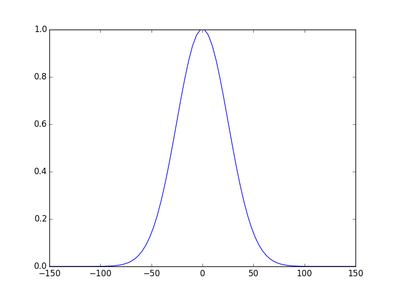
Well nothing new till now this is basically tutorial2, and as we just explained the mode shown by the solver is the mode inside the cavity on the first mirror. To calculate the output beam say at 5cm outside the cavity first we have to define the ABCD matrix of the optical system shown in the figure below:
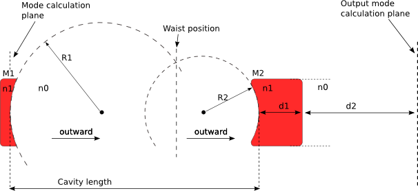
The ABCD matrix of this optical system can be written as follows:
As you can notice the order of matrix multiplication is inverted, so from the first plane on the first mirror M1 to the final plane outside the optical cavity where we want to calculate the output beam we have: Propagation distance Lc, then refraction at curved interface (n0/n1), propagation distance d1, refraction at flat interface and finally propagation distance d2 until the final plane. let’s enter this matrices and calculate the global matrix system by taking n0=1, n1=1.5, and d1=5mm, and d2=50mm. We also calculate the global matrix in the case of free space propagation by neglecting the mirror M2 to see its effect on the output beam.
In [9]: M00=ms.np.array([[1,Lc ],[0, 1]]);

In [10]: M01=ms.np.array([[1,0 ],[(1-1.5)/(-R2*1.5), 1/1.5]]);# -R2  (<0 because it is a concave interface)

In [11]: M02=ms.np.array([[1,5e3 ],[0, 1]]);

In [12]: M03=ms.np.array([[1,1 ],[0, 1.5/1]]);

In [13]: M04=ms.np.array([[1,50e3 ],[0, 1]]);

In [14]: M_out=M04.dot(M03.dot(M02.dot(M01.dot(M00))));

In [15]: M_out2=ms.np.array([[1,Lc+5e3+50e3 ],[0, 1]]); # neglecting M2 = just propagation distances
Now that the matrices are calculated, we will create a Fresnel propagator object then set the propagation system and the beam to propagate for each case
(with / without the concave mirror M2) then we use propagate1D_ABCD() function to propagate the beam.
In [16]: from opencavity.propagators import FresnelProp

In [17]: propsys=FresnelProp() #create propagator object

In [18]: propsys2=FresnelProp()

In [19]: l,tem00=opsys.get_mode1D(0) # get the fundamental mode of the cavity

In [20]: propsys.set_start_beam(tem00, opsys.x1) # set the beam to propagate

In [21]: propsys2.set_start_beam(tem00, opsys.x1)

In [22]: propsys.set_ABCD(M_out) # taking M2 into account

In [23]: propsys2.set_ABCD(M_out2) # without M2

In [24]: propsys.propagate1D_ABCD(x2=10*opsys.x1) # calculate the propagation from initial plane to a plane 10 times larger (the beam is wider)

In [25]: propsys2.propagate1D_ABCD(x2=10*opsys.x1)

In [26]: propsys.show_result_beam(what='intensity') # show propagation result

In [27]: propsys2.show_result_beam(what='intensity')
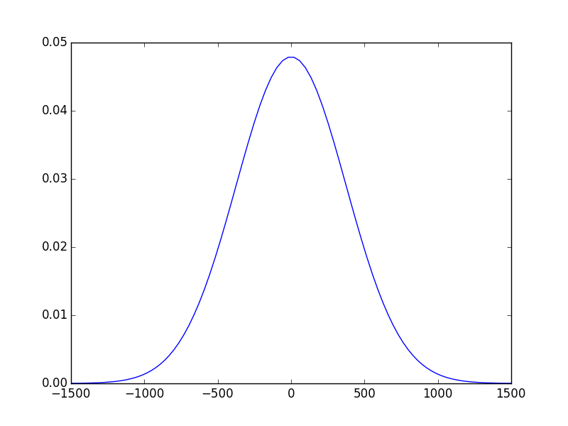
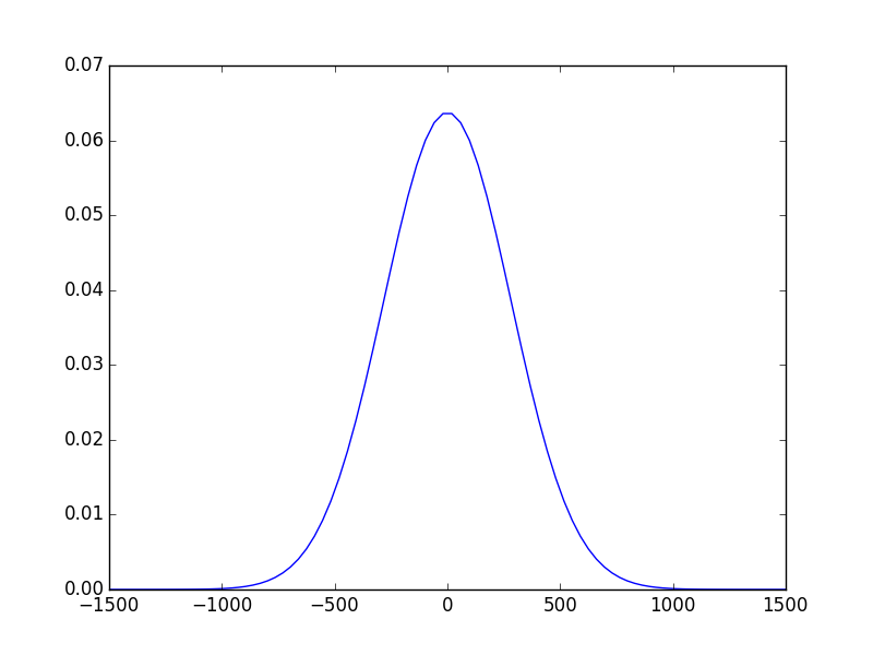
What we can see from comparing these two figures is that when the beam propagates trough the output mirror it diverges more than in the case of pure
free space propagation, actually the output mirror acts like a diverging lens and this is not surprising given its shape.
For a more precise comparison we can get the waist of the beam using the function find_waist(beam,x) in the class CavEigenSys before this we have to get the result beam using
the function get_result_beam() in the class FresnelProp as follows:
In [28]: tem00_1,x=propsys.get_result_beam() # get the propagated beam and the abscissa vector

In [29]: tem00_2,x=propsys2.get_result_beam()

In [30]: print opsys.find_waist(tem00_1,x) # calculate the waist of the beam at 36% of maximum amplitude
797.449863496

In [31]: print opsys.find_waist(tem00_2,x)
589.789316892
The cleaned code
# -*- coding: utf-8 -*-
'''

@author: M.seghilani
'''

import opencavity.modesolver as ms
from opencavity.propagators import FresnelProp

R1=1e13; R2=10*1e3; Lc=8*1e3; npts=120; a=150; # cavity parameters
g1=1-Lc/R1; g2=1-Lc/R2;
A=2*g1*g2-1; B=2*g2*Lc; C=2*g1/Lc; D=2*g1*g2-1;

opsys=ms.CavEigenSys();
opsys.build_1D_cav_ABCD(a,npts,A,B,C,D)
opsys.solve_modes()
opsys.show_mode(0)
#opsys.show_mode(2,what='intensity')
opsys.show_mode(0,what='phase')
ms.plt.show()

# creating ABCD matrix of the beam path from the mode calculation plane to the output calculation plane
M00=ms.np.array([[1,Lc ],[0, 1]]);
M01=ms.np.array([[1,0 ],[(1-1.5)/(-R2*1.5), 1/1.5]]);
M02=ms.np.array([[1,5e3 ],[0, 1]]);
M03=ms.np.array([[1,1 ],[0, 1.5/1]]);
M04=ms.np.array([[1,50e3 ],[0, 1]]);

M_out=M04.dot(M03.dot(M02.dot(M01.dot(M00)))); # global matrix
M_out2=ms.np.array([[1,Lc+5e3+50e3 ],[0, 1]]); # free space ABCD system from mode calculation plane to output calculation plane

l,tem00=opsys.get_mode1D(0)

propsys=FresnelProp() # create a propagator object
propsys2=FresnelProp()
propsys.set_start_beam(tem00, opsys.x1)
propsys2.set_start_beam(tem00, opsys.x1)
propsys.set_ABCD(M_out) # set the propagation matrix
propsys2.set_ABCD(M_out2)

propsys.propagate1D_ABCD(x2=10*opsys.x1) # propagate the beam
propsys2.propagate1D_ABCD(x2=10*opsys.x1)

propsys.show_result_beam(what='intensity') # show the propagated beam
propsys2.show_result_beam(what='intensity')

tem00_1,x=propsys.get_result_beam()# fetch propagated beam and abscissa
tem00_2,x=propsys2.get_result_beam()

print opsys.find_waist(tem00_1,x) # find the wais of the beam
print opsys.find_waist(tem00_2,x)

ms.plt.show()