Tutorial 8 - 2D cavity with masks
In this tutorial we learn how to use OpenCavity to design 2D cavities with masks as we did for 1D case in Tutorial 3 - using apertures and phase masks. The procedure is quite similar, and as 2D masks can be more complicated to generate than 1D ones OpenCavity comes with mask generation class called AmpMask2D() that can be used to create a mask object and modify it, then we can apply this mask object to a given cavity system using the function apply_mask2D() as we will see. Of course you can just create a mask object using a given phase or amplitude function as we did in 1D case than apply it to the system the AmpMask2D() class is here just to simplify the creation of some usual amplitude masks as an aperture for example.
Lets start by creating the cavity system:
In [1]: import opencavity.modesolver as ms; #importing the opencavity module

In [2]: import matplotlib.pylab as plt

In [3]: import numpy as np

In [4]: sys=ms.CavEigenSys() #creating a ms object

In [5]: R1=1e13; R2=10*1e3; Lc=8*1e3; npts=64; a=80; # cavity parameters

In [6]: g1=1-Lc/R1; g2=1-Lc/R2; # g1 and g2 parameters of the cavity

In [7]: A1=2*g1*g2-1; B1=2*g2*Lc; C1=2*g1/Lc; D1=2*g1*g2-1; # ABCD elements written using g1,g2

In [8]: sys.build_2D_cav_ABCD(a, npts, A1,B1,C1,D1) # building the cavity
Building the  kernel matrix ...
Building the  kernel matrix done.
We use now AmpMask2D() class to create and show the mask, but before this we need to get the discretized grid of the cavity system in which we build
the mask, keep in mind that in OpenCavity all spatial entities are not linearly spaced, see :ref: vector-spacing-label for more details.
In [9]: x1=sys.x1; y1=sys.y1
In [10]: apert=ms.AmpMask2D(x1,y1) # create a mask object
creating mask object...
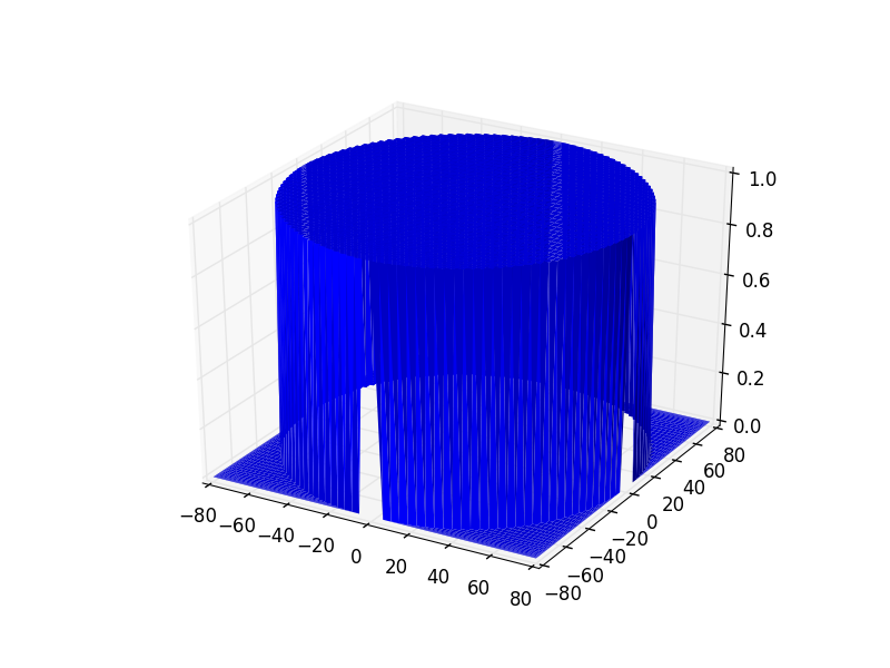
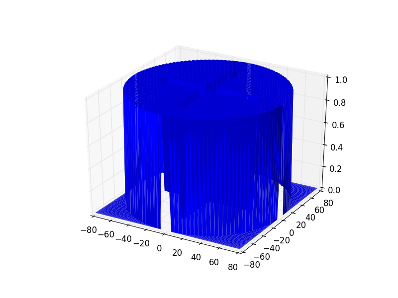
In [11]: apert.add_circle(80) #create an aperture in x1,y1 coordinates with radius=80
In [12]: apert.show_msk3D() # plot the mask function to check the created distribution
Now we know what the mask looks like, let’s apply it to the cavity system and calculate the modes.
In [13]: sys.apply_mask2D(apert) # apply the mask to the system (1st plane)
Applying 2D Mask...
Mask applied.
In [14]: sys.solve_modes()
running the eigenvalues solver...
#show some modes
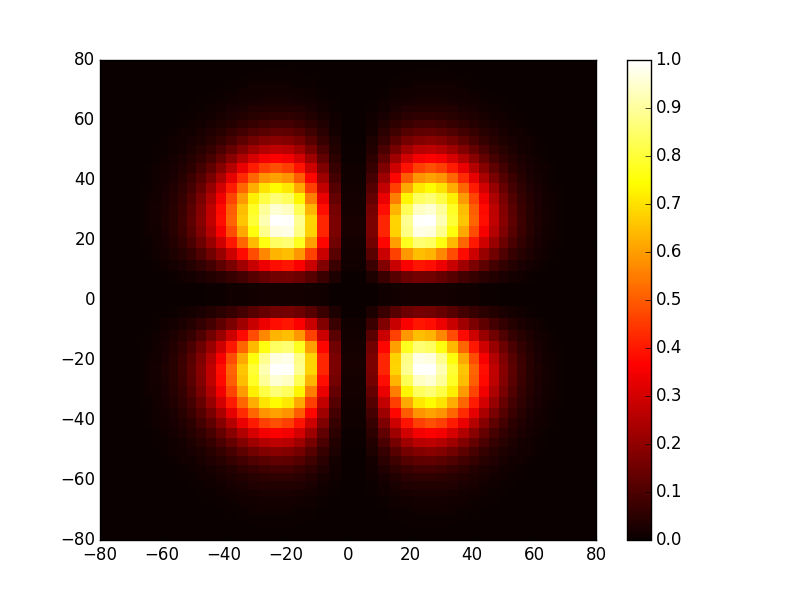
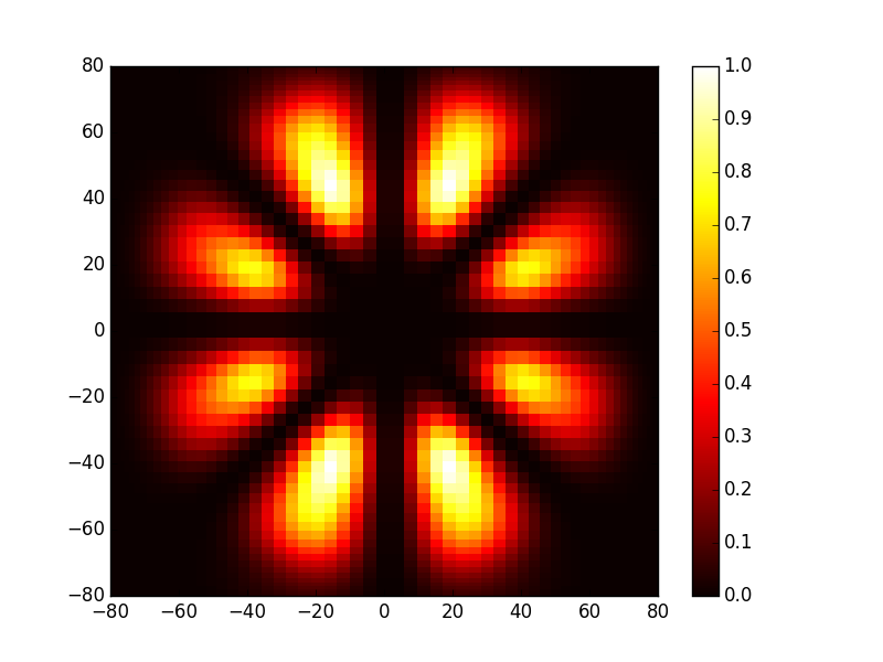
In [15]: plt.set_cmap('hot')
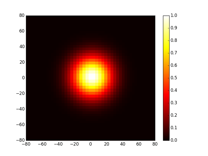
In [16]: sys.show_mode(0,what='intensity')
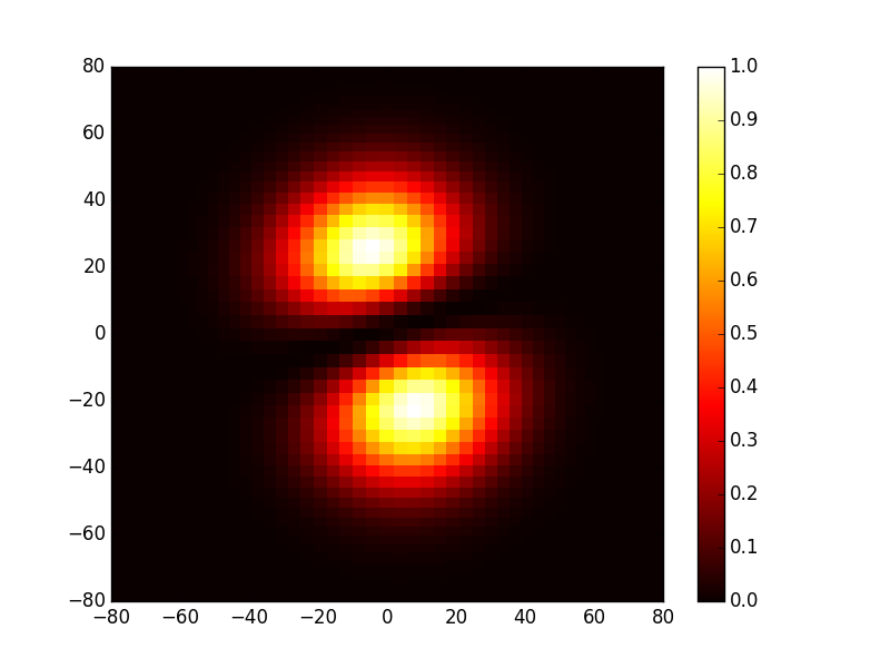
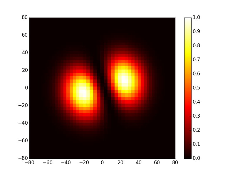
In [17]: sys.show_mode(1,what='intensity')
In [18]: sys.show_mode(2,what='intensity')
In [19]: sys.show_mode(3,what='intensity')

Lets add some modifications to the amplitude mask and see what impact it has on the eigenmodes
In [20]: x1=sys.x1; y1=sys.y1

In [21]: apert.add_rectangle(2, 50,positive='False') # a lossy rectangle (amplitude =0)

In [22]: apert.add_rectangle(50, 2,positive='False')

In [23]: apert.show_msk3D()
This mask is supposed to introduce losses in the dark region of the mode TEM11, so this latter will be the less affected by this mask thus we expect it to become the first mode (having the biggest eigenvalue) of this cavity, let’s check this.
In [24]: sys.apply_mask2D(apert)
Applying 2D Mask...
Mask applied.

In [25]: sys.solve_modes()
running the eigenvalues solver...

In [26]: sys.show_mode(0,what='intensity')

In [27]: sys.show_mode(1,what='intensity')

In [28]: sys.show_mode(2,what='intensity')
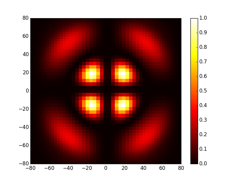
The three first modes of this cavity have zero intensity region that falls in the lossy region of the mask as we expected. let’s take a look at the eigenvalue:
In [29]: l,tem00=sys.get_mode2D(0);

In [30]: print 1-np.abs(l)**2 #round trip losses
0.0128670609823
The cleaned code
# -*- coding: utf-8 -*-
'''

@author: M.seghilani
'''

import opencavity.modesolver as ms

R1=1e13; R2=10*1e3; Lc=8*1e3; npts=64; a=80; # cavity parameters
g1=1-Lc/R1; g2=1-Lc/R2;
A1=2*g1*g2-1; B1=2*g2*Lc; C1=2*g1/Lc; D1=2*g1*g2-1;
sys=ms.CavEigenSys() #creating a ms object
sys.build_2D_cav_ABCD(a, npts, A1,B1,C1,D1)

x1=sys.x1; y1=sys.y1

apert=ms.AmpMask2D(x1,y1) # create a mask object
apert.add_circle(80)#create an aperture in x1,y1 coordinates with radius=80
apert.show_msk3D()
sys.apply_mask2D(apert)

sys.solve_modes()
sys.show_mode(0)
sys.show_mode(1)
sys.show_mode(2)

# add two crossed lossy lines at the center of the mask
apert.add_rectangle(2, 50,positive='False')
apert.add_rectangle(50, 2,positive='False')
apert.show_msk3D()
sys.apply_mask2D(apert)

sys.solve_modes()
sys.show_mode(0,'intensity')
sys.show_mode(1,'intensity')
sys.show_mode(2,'intensity')


ms.plt.show()