Tutorial 1 - Simple 2 mirror cavity

System definition

In this example we see how to calculate the eigenmodes of a simple 2 mirrors optical resonator (see Fig below)

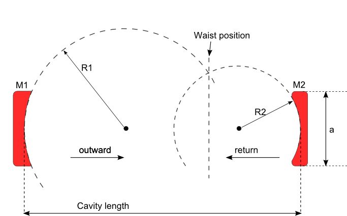
Where M1, M2 are two mirrors with radius of curvature R1,R2 respectively, and Lc the distance between M1,M2 is the cavity length. It is important to note that the sign convention adopted is R>0 means concave mirror and R<0 means a convex one. We consider a plano-concave cavity also called VECSEL type cavity, for Vertical Cavity Surface Emitting lasers which means that the waist is on the plane mirror.

This is the simplest example one can get, Well let’s see how to calculate the eigenmodes of this cavity:

In [1]: import opencavity.modesolver as ms; #importing the opencavity module

#creating an empty system at wavelength =1.01, this will contain all the problem parameters
In [2]: sys=ms.CavEigenSys(wavelength=1.01);

In [3]: R1=1e13; R2=10*1e3; Lc=8*1e3; npts=120; a=150; # defining the cavity parameters

In [4]: sys.build_1D_cav(a, npts, R1, R2, Lc); # building the matrix-kernel system
Building the  kernel matrix ...
Building the  kernel matrix done.

In [5]: sys.solve_modes(n_modes=10); # solve the 10 first modes of the cavity, default value of n_modes is 30
running the eigenvalues solver...

• in the first command we import the CavityMode module and we call it ms in the running session, the ; is used to not show messages.

• in the command 2 we create a opencavity object working at a wavelength=1.01, this object will contain all the system (parameters, solutions...) note that:

  • the default wavelength is 1, this means that sys=ms.CavEigenSys() = sys=ms.CavEigenSys(wavelength=1)
  • the wavelength is unitless, thus all distances are in the wavelength unit. (here we consider micron)

• in line 3 we just enter the cavity parameters.

• in line 4 we build the Fresnel-kernel matrix of the system.

• in line 5 we ask the solver to find the 10 first eigenvalues and modes of the cavity in ‘sys’, note that

  • the default value of n_modes is 30.

Now to see the calculated modes and eigenvalues:

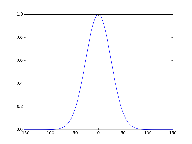
In [6]: sys.show_mode(0); #plot the E-field of the 1st mode.

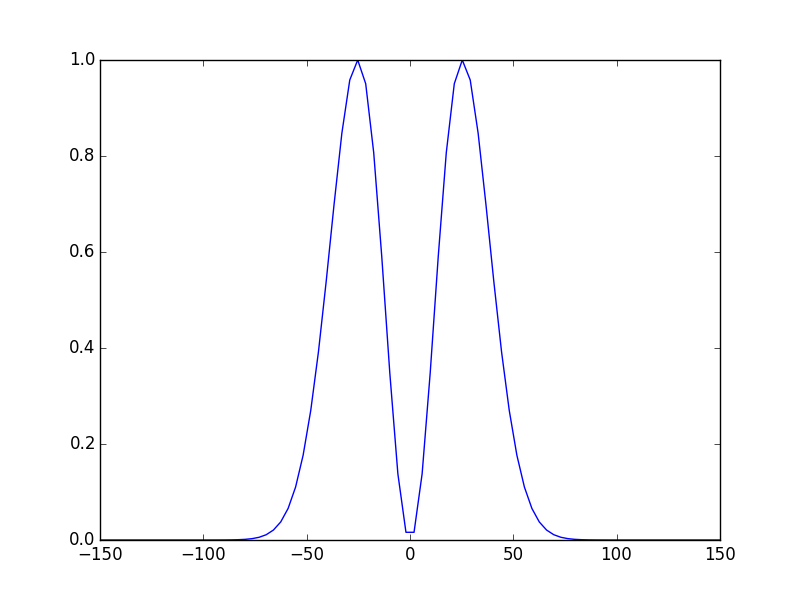
In [7]: sys.show_mode(1,what='intensity'); #plot the intensity of the 2d mode.

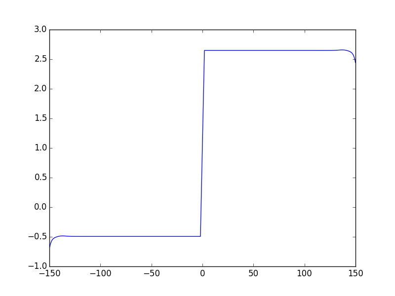
In [8]: sys.show_mode(1,what="phase");  #plot the phase of the 2nd mode.

The calculated eigenmodes and eigenvalues are in sys, to get them:

In [9]: l,v=sys.get_mode1D(0) # l is the eigenvalue, and v the eigenvector: complex E-field of the mode

In [10]: print(1-ms.np.abs(l)**2) # the round trip losses = 1- |l|^2, we use np numerical-python imported within the ms
0.0099009900994

In this example we used the function buid_1D_cav() to build the cavity kernel, this function is appropriate for simple systems like the one of this tutorial when we have linear 2 mirrors cavity. However, there is a more general and powerful function which is build_1D_cav_ABCD() which can be used to define any optical cavity using its transfer matrix. (see Gaussian optics and paraxial ray matrices). In the forthcoming tutorials we will use this function, including the next one which is a tutorial that aim at getting familiar with defining general cavity designs.

To summarize, the steps one should do to define a cavity systems and find its modes using opencavity can be summarized as follows:

• importing opencavity module
• enter the cavity parameters
• create a solver object (CavEigenSys()) that keeps in one place all informations about the system
• solve the mode
• show the modes

To end, we note that there are two very useful features when using spyder: auto-completion by hitting tab key after the point, such as for sys., this gives all the available functions in the class. And when you are not sure how to use a given function, you can hit Ctl+i to show the function help in the object inspector.

The cleaned code

# -*- coding: utf-8 -*-

import opencavity.modesolver as ms

sys=ms.CavEigenSys() #creating a ms object
R1=1e13; R2=10*1e3; Lc=8*1e3; npts=120; a=150; # cavity parameters 

sys.build_1D_cav(a, npts, R1, R2, Lc) # build the system
sys.solve_modes() #solve the modes default n_modes=30

sys.show_mode(0) #plots the E-field of the 1st mode 

sys.show_mode(1,what='intensity') #plots the intensity of the 2nd mode
sys.show_mode(1,what='phase') #plots the phase of the 2nd mode
ms.plt.show()

l,v=sys.get_mode1D(0) #l: eigenvalue; v: eigenmode